Running a Spin-Boson Model#
Here’s a simple example of how to run a spin-boson model with mean-field dynamics (also known as Ehrenfest dynamics) in QC Lab. A Jupyter Notebook version of this tutorial can be found here.
First, we will need to import the necessary modules:
import numpy as np
import matplotlib.pyplot as plt
from qclab import Simulation
from qclab.models import SpinBoson
from qclab.algorithms import MeanField
from qclab.dynamics import serial_driver
Next, we will set up the Simulation object and equip it with the Model and Algorithm objects:
# Initialize the Simulation object.
sim = Simulation()
# Equip it with a spin-boson Model object.
sim.model = SpinBoson()
# Attach the mean-field algorithm.
sim.algorithm = MeanField()
# Initialize the diabatic wavefunction.
# Here, the first vector element refers to the upper state and the second
# element refers to the lower state.
sim.initial_state["wf_db"] = np.array([1, 0], dtype=complex)
This is bound to run the spin-boson model using default values for the model constants.
Following the definitions from Tempelaar & Reichman 2019, the model constant
values are kBT=1.0, E=0.5, V=0.5, A=100, W=0.1, and l_reorg=0.005 (which can be found here).
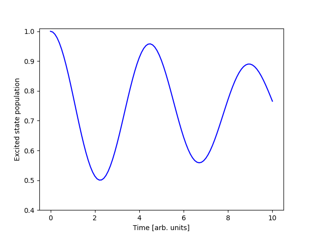
Finally, we can run the simulation and visualize the results:
# Run the simulation.
data = serial_driver(sim)
# Pull out the time.
t = data.data_dict["t"]
# Get populations from the diagonal of the density matrix.
populations = np.real(np.einsum("tii->ti", data.data_dict["dm_db"]))
plt.plot(t, populations[:, 0], color="blue")
plt.xlabel('Time [arb. units]')
plt.ylabel('Excited state population')
plt.ylim([0.4,1.01])
plt.show()
The output of this code is:
Note
This simulation ran in serial mode. For a speed-up on high-performance architecture, consider adopting a parallel Dynamics Driver,
e.g. data = parallel_driver_multiprocessing(sim). More information on parallelization can be found in the
Drivers section.
I want to increase the reorganization energy.#
Changing the reorganization energy is easy! Using the same Simulation object from the previous example, we can modify the l_reorg constant in sim.model.constants:
sim.model.constants.l_reorg = 0.05
The output changes to (dash shows previous result):
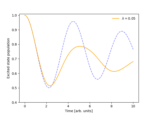
For the full set of Model object constants, see the Spin-Boson Model section.
I want to use FSSH instead.#
Sure! Following the previous example, swap sim.algorithm to FewestSwitchesSurfaceHopping:
from qclab.algorithms import FewestSwitchesSurfaceHopping

sim.algorithm = FewestSwitchesSurfaceHopping()
The output has changed once more:
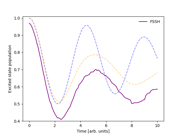
You can learn about algorithms in the Algorithms section.
Note
The populations above are not in agreement at the outset of the simulation because the FSSH algorithm stochastically samples the initial state while the mean-field algorithm does not. If the number of trajectories were increased, the initial populations would converge to the same value.
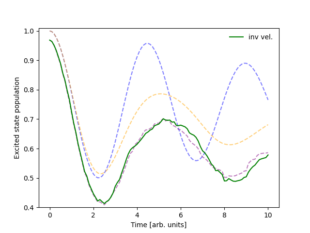
I want to reverse velocities upon frustrated hops.#
Let’s try modifying the FSSH Algorithm object so that the velocities of frustrated trajectories are reversed. In the complex coordinate formalism, this means conjugating the z coordinate of the frustrated trajectories. To this end, we write the following function:
def update_z_reverse_frustrated_fssh(sim, state, parameters):
    """
    Reverse the velocities of frustrated trajectories in the FSSH algorithm.
    """
    # Get the indices of trajectories that were frustrated
    # (i.e., did not successfully hop but were eligible to hop).
    frustrated_indices = state["hop_ind"][~state["hop_successful"]]
    # Reverse the velocities for these indices, in the complex classical coordinate
    # formalism, this means conjugating the z coordinate.
    state["z"][frustrated_indices] = state["z"][frustrated_indices].conj()
    return state, parameters
Now we can insert this function as a Task into an instance of the FSSH Algorithm object. To know where we should insert it, we can look
at the update_recipe of the FSSH Algorithm object (see Surface Hopping Example).
A good place to invert the velocities of frustrated trajectories is just at the end of the active surface updates. We append the new Task to the end of the update Recipe using a standard Python list method:
# Insert the function for reversing velocities as a task into the update recipe.
sim.algorithm.update_recipe.append(update_z_reverse_frustrated_fssh)
The output has now changed to:
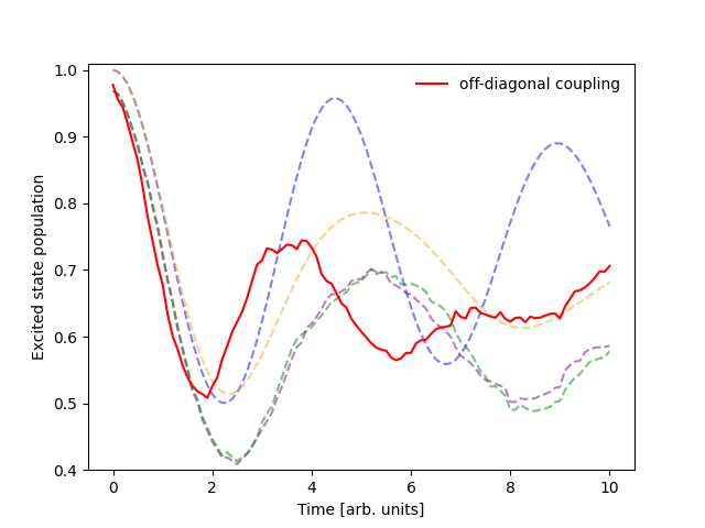
I want to switch to off-diagonal coupling.#
Changing the coupling term is straightforward! We’ll make a new Ingredient that couples the boson coordinates to the off-diagonal elements of the quantum Hamiltonian.
For simplicity we will make an Ingredient that creates the quantum-classical interaction Hamiltonian for a single trajectory and then use QC Lab’s built-in vectorization decorator to automatically vectorize it.
from qclab.functions import vectorize_ingredient

@vectorize_ingredient
def h_qc(model, parameters, **kwargs):
    """
    A coupling term that couples the boson coordinates to the off-diagonal elements of the quantum Hamiltonian.
    """
    # First we'll get the z coordinate from the keyword arguments
    z = kwargs['z']
    # Next we'll get the Required constants from the constants object.
    m = model.constants.classical_coordinate_mass
    h = model.constants.classical_coordinate_weight
    g = model.constants.harmonic_frequency * np.sqrt(2 * model.constants.l_reorg / model.constants.A)
    # Now we can construct the empty Hamiltonian matrix as a 2x2 complex array.
    h_qc = np.zeros((2, 2), dtype=complex)
    # Then we can populate the off-diagonal elements of the Hamiltonian matrix.
    h_qc[0, 1] = np.sum((g * np.sqrt(1 / (2 * m * h))) * (z + np.conj(z)))
    h_qc[1, 0] = np.conj(h_qc[0, 1])
    return h_qc
Next, we add the new Ingredient to the Model object’s ingredients list and override the analytical gradient Ingredient (which is no longer correct for the new coupling). QC Lab will then differentiate the new coupling term numerically using finite differences.
# Add the new coupling term to the Model object's Ingredients.
sim.model.ingredients.append(("h_qc", h_qc))
# Overwrite the analytical gradient Ingredient, which is no longer correct for the new coupling.
sim.model.ingredients.append(("dh_qc_dzc", None))
Now we can run the simulation with the new coupling term and compare the results to the previous simulation. You’ll notice a small decrease in the performance of the simulation due to the numerical calculation of the gradients. If you’d like to speed up the simulation, you can implement an analytical gradient for the new coupling term by following the Sparse Quantum-Classical Gradients section.
Putting it all together.#
This is what the final code looks like:
import numpy as np
import matplotlib.pyplot as plt
from qclab import Simulation
from qclab.models import SpinBoson
from qclab.algorithms import FewestSwitchesSurfaceHopping
from qclab.dynamics import serial_driver
from qclab.functions import vectorize_ingredient

def update_z_reverse_frustrated_fssh(sim, state, parameters):
    """
    Reverse the velocities of frustrated trajectories in the FSSH algorithm.
    """
    # Get the indices of trajectories that were frustrated
    # (i.e., did not successfully hop but were eligible to hop).
    frustrated_indices = state["hop_ind"][~state["hop_successful"]]
    # Reverse the velocities for these indices, in the complex classical coordinate
    # formalism, this means conjugating the z coordinate.
    state["z"][frustrated_indices] = state["z"][frustrated_indices].conj()
    return state, parameters

@vectorize_ingredient
def h_qc(model, parameters, **kwargs):
    """
    A coupling term that couples the boson coordinates to the off-diagonal elements of the quantum Hamiltonian.
    """
    # First we'll get the z coordinate from the keyword arguments
    z = kwargs['z']
    # Next we'll get the Required constants from the constants object.
    m = model.constants.classical_coordinate_mass
    h = model.constants.classical_coordinate_weight
    g = model.constants.harmonic_frequency * np.sqrt(2 * model.constants.l_reorg / model.constants.A)
    # Now we can construct the empty Hamiltonian matrix as a 2x2 complex array.
    h_qc = np.zeros((2, 2), dtype=complex)
    # Then we can populate the off-diagonal elements of the Hamiltonian matrix.
    h_qc[0, 1] = np.sum((g * np.sqrt(1 / (2 * m * h))) * (z + np.conj(z)))
    h_qc[1, 0] = np.conj(h_qc[0, 1])
    return h_qc

# Initialize the Simulation object.
sim = Simulation()
# Equip it with a spin-boson Model object.
sim.model = SpinBoson()
# Change the reorganization energy.
sim.model.constants.l_reorg = 0.05
# Add the new coupling term to the model's ingredients.
sim.model.ingredients.append(("h_qc", h_qc))
# Overwrite the analytical gradient ingredient, which is no longer correct for the new coupling.
sim.model.ingredients.append(("dh_qc_dzc", None))
# Attach the FSSH algorithm.
sim.algorithm = FewestSwitchesSurfaceHopping()
# Insert the function for reversing velocities as a task into the update recipe.
sim.algorithm.update_recipe.append(update_z_reverse_frustrated_fssh)
# Initialize the diabatic wavevector.
# Here, the first vector element refers to the upper state and the second
# element refers to the lower state.
sim.initial_state["wf_db"] = np.array([1, 0], dtype=complex)

# Run the simulation.
data = serial_driver(sim)

# Pull out the time.
t = data.data_dict["t"]
# Get populations from the diagonal of the density matrix.
populations = np.real(np.einsum("tii->ti", data.data_dict["dm_db"]))
plt.plot(t, populations[:, 0], color="red")
plt.xlabel('Time [arb. units]')
plt.ylabel('Excited state population')
plt.ylim([0.4,1.01])
plt.savefig("full_code_output.png")
plt.show()