Quick Start Guide#
QC Lab is organized into models and algorithms which are combined into a simulation object. The simulation object fully defines a quantum-classical dynamics simulation which is then carried out by a dynamics driver. This guide will walk you through the process of setting up a simulation object and running a simulation.
The code in this page is implemented in the notebook quickstart.ipynb which can be found in the examples directory of the repository.
Importing Modules#
First, we import the necessary modules.
import numpy as np
import matplotlib.pyplot as plt
from qc_lab import Simulation # import simulation class
from qc_lab.models import SpinBoson # import model class
from qc_lab.algorithms import MeanField # import algorithm class
from qc_lab.dynamics import serial_driver # import dynamics driver
Instantiating Simulation Object#
Next, we instantiate a simulation object from qc_lab.Simulation. Each object has a set of default settings which can be accessed by calling sim.default_settings. Passing a dictionary to the simulation object when instantiating it will override the default settings.
sim = Simulation()
print('default simulation settings: ', sim.default_settings)
# default simulation settings:  {'tmax': 10, 'dt': 0.01, 'dt_output': 0.1, 'num_trajs': 10, 'batch_size': 1}
Alternatively, you can directly modify the simulation settings by assigning new values to the settings attribute of the simulation object. Here we change the number of trajectories that the simulation will run, and how many trajectories are run at a time (the batch size). We also change the total time of each trajectory (tmax) and the timestep used for propagation (dt).
Note
QC Lab expects that the total time of the simulation (tmax) is an integer multiple of the output timestep (dt_output), which must also be an integer multiple of the propagation timestep (dt).
# change settings to customize simulation
sim.settings.num_trajs = 200
sim.settings.batch_size = 50
sim.settings.tmax = 30
sim.settings.dt = 0.01
sim.settings.dt_output = 0.1
Instantiating Model Object#
Next, we instantiate a model object. Like the simulation object, it has a set of default constants.
sim.model = SpinBoson()
print('default model constants: ', sim.model.default_constants)
# default model constants:  {'temp': 1, 'V': 0.5, 'E': 0.5, 'A': 100, 'W': 0.1, 'l_reorg': 0.005, 'boson_mass': 1}
Instantiating Algorithm Object#
Next, we instantiate an algorithm object which likewise has a set of default settings.
sim.algorithm = MeanField()
print('default algorithm settings: ', sim.algorithm.default_settings)
# default algorithm settings:  {}
Setting Initial State#
Before using the dynamics driver to run the simulation, it is necessary to provide the simulation with an initial state. This initial state is dependent on both the model and algorithm. For mean-field dynamics, we require a diabatic wavefunction called “wf_db”. Because we are using a spin-boson model, this wavefunction should have dimension 2. The initial state is stored in sim.state which can be accessed as follows.
sim.state.wf_db = np.array([1, 0], dtype=complex)
Running the Simulation#
Finally, we run the simulation using the dynamics driver. Here, we are using the serial driver. QC Lab comes with several different types of parallel drivers which are discussed elsewhere.
data = serial_driver(sim)
Analyzing Results#
The data object returned by the dynamics driver contains the results of the simulation in a dictionary with keys corresponding to the names of the observables that were requested to be recorded during the simulation.
print('calculated quantities:', data.data_dict.keys())
# calculated quantities: dict_keys(['seed', 'dm_db', 'classical_energy', 'quantum_energy'])
Each of the calculated quantities is normalized with respect to the number of trajectories (note that this might depend on the type of algorithm used) and can be accessed through the data.data_dict attribute. The normlaization factor for the data is kept in data.data_dict[“norm_factor”].
norm_factor = data.data_dict['norm_factor']
classical_energy = data.data_dict['classical_energy']
quantum_energy = data.data_dict['quantum_energy']
populations = np.real(np.einsum('tii->ti', data.data_dict['dm_db']))
The time axis can be retrieved from the simulation object through its settings.
time = sim.settings.tdat_output
Plotting Results#
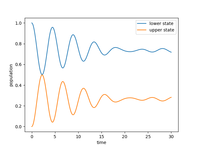
Finally, we can plot the results of the simulation like the population dynamics.
plt.plot(time, populations[:, 0], label='upper state')
plt.plot(time, populations[:, 1], label='lower state')
plt.xlabel('time')
plt.ylabel('population')
plt.legend()
plt.show()
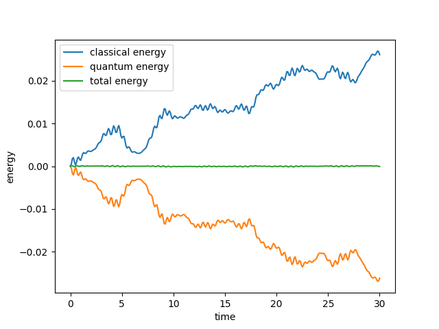
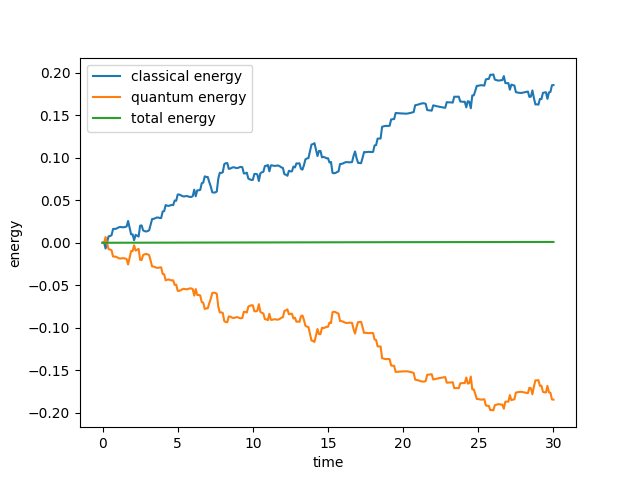
We can verify that the total energy of the simulation was conserved by inspecting the change in energy of quantum and classical subsystems over time.
plt.plot(time, classical_energy - classical_energy[0], label='classical energy')
plt.plot(time, quantum_energy - quantum_energy[0], label='quantum energy')
plt.plot(time, classical_energy + quantum_energy - classical_energy[0] - quantum_energy[0], label='total energy')
plt.xlabel('time')
plt.ylabel('energy')
plt.legend()
plt.show()
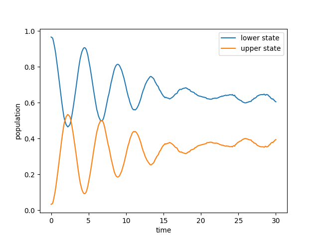
Changing the Algorithm#
If you want to do a surface hopping calculation rather than a mean-field one, QC Lab makes it very easy to do so. Simply import the relevant Algorithm class and set sim.algorithm to it and rerun the calculation.
from qc_lab.algorithms import FewestSwitchesSurfaceHopping

sim.algorithm = FewestSwitchesSurfaceHopping()

data = serial_driver(sim)
The populations can be visualized in a similar way as before. Note that the simulation settings chosen here are solely for testing purposes. Publication quality simulations would require checking convergence of the number of trajectories and the timestep.
Changing the Driver#
You can likewise run the simulation using a parallel driver. Here we use the multiprocessing driver to split the trajectories over four tasks.
from qc_lab.dynamics import parallel_driver_multiprocessing

data = parallel_driver_multiprocessing(sim, num_tasks=4)
Units in QC Lab#
QC Lab is written assuming all energies are in units of the thermal quantum (\(k_{\mathrm{B}}T\)). Units of time are then determined by assuming a value for the temperature defining the thermal quantum and calculating the equivalent timescales. For example, if we assume a standard temperature of \(T = 298.15\,\mathrm{K}\) then the thermal quantum is \(k_{\mathrm{B}}T = 25.7\,\mathrm{meV}\) and one unit of time is \(\hbar/k_{\mathrm{B}}T = 25.6\,\mathrm{fs}\).